R for Biophysical Chemists
This page is a work in progress, in support of Chem 728, Physical Biochemistry, offered by Craig Martin in Spring 2021 at the University of Massachusetts Amherst. It is offered to highlight the narrow set of features in R that are important for concepts developed in this course.
Quick navigation: Basics, Functions, Curve Fitting, Plotting, Importing Data, Files
The R Project for Statistical Computing (or just R) is freely available on essentially all platforms. It is command line driven, but can do complex analyses and create beautiful output. Start by downloading (from a local server) the version of R for your computer. The introduction below will tell us how to manipulate data, create functions, fit data to functions, import data from a file, plot the data and function, and output the plot to a file.
[ I highly recommend that you instead download the program RStudio (the free version works well: RStudio Desktop - Open Source Edition), that provides an integrated environment for R. The command environment, plots, and other optional things can all be viewed in different parts of one window (I may use this in class for easier sharing of the one window). All of the commands are identical, but some commands are also available from a conventional menu. ]
Basic Information
File locations. Mostly, we'll want to read data from a text file, and we'll want to export data, plots, and sessions to files. The first concept is the working directory. By default, R will set your "root" directory as the working directory. To find out what that current "path" is, type the following at the command line (followed by return): getwd(). The result might be something like /Users/janedoe"
To set your desktop as the working directory, use setwd("~/Desktop"), (where ~ refers to your default "root" directory, /Users/janedoe), above. To make sure you are in the right place, list.files() will list all of the files in R's current directory. Finally, although not essential, avoid spaces or special characters in file names [note that setting the working directory is a menu option in RStudio: Session > Set Working directory].
Be sure that all quotation marks used are "straight" quotes, rather than "curly" quotes.
Objects. Data are placed into vector objects, as in any programming language. For example, the following creates objects that contain data:
t <- 0:20
y <- exp(-t/2)
The first command above creates an integer series 0, 1, 2, ... 20 and loads it into a new variable t (to generate a series 1.1, 1.2, ... 2.4, 2.5 use seq(1.1, 2.5, 0.1)). The second command creates an exponential decay series from the series data in the object t and loads it into y. Note that these expressions can also be written in the more traditional formalism: t = 0:20 and y = exp(-t/2), but we'll try and keep to the more readable R formalism.
t and y are now "vectors" (a series of values, also known as lists or arrays in other languages). Think of a column of data in Excel as a vector (indeed, we'll learn below how to read an Excel data column into an R (vector) variable).
The command line. One very useful thing to know is that recent commands are stored and can be retrieved by use of the up arrow key. Bring back a previous command, edit it, and then hit return to execute the edited command.
Quick navigation: Basics, Functions, Curve Fitting, Plotting, Importing Data, Files
User functions in R
In this course, we will fit data to mechanistic models that are represented mathematically. We don't want to use a canned (black box) function; we want to use our own function, corresponding to a mechanistic model we are testing. To define a more general exponential decay function in R, we could use:
myExpDecay <- function(texpt, ampl, tau, shft) (shft +(ampl*(exp(-texpt/tau))))
In this function definition, the first parameter in the first set of parentheses is experimental time (our x-value), while the remaining are the function parameters amplitude (ampl), lifetime (tau), and baseline offset (shft). Within the second set of parentheses is the function definition, which follows simple algebraic logic using the given parameters. After defining the function, you can then use:
ExpData <- myExpDecay(t, 5.0, 4.2, 10.0)
Since t is a vector, ExpData will now be a similar vector, but with the exponential decay data loaded into corresponding positions in the vector.
ExpData <- myExpDecay(t,5.0,8.0,10.0) + rnorm(21,mean=0,sd=0.2)
In this case, we use our function, along with the built-in function rnorm to generate "normally distributed" random numbers, to generate "data" with fictitious noise. We'll learn about plot(x,y) in a minute, but to see how this works, type the following (remember that we defined t above):
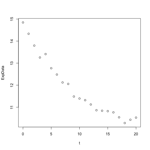
plot(t, ExpData)
You should see a scatter plot of of 21 data points, following an exponential decay. We're now ready to use myExpDecay both to generate some "experimental" data and to fit that data using nonlinear least squares regression.
Quick navigation: Basics, Functions, Curve Fitting, Plotting, Importing Data, Files
Plotting
Plotting data. There are various plotting "packages" available in R. One of the more feature-rich is ggplot2, but it requires installation and has a steep learning curve. The following describes the use of the primary plotting tool available in the basic install - plot(x,y).
For a simple plot of decay vs time from the above data (remember that we defined t above), use:
plot(t, ExpData)
This should give you a plot as shown here. Remember that t and ExpData are the equal length vectors we defined above.
There are many (optional) options for this command. For example, the above defaults to plotting symbols for each data point.
Plotting curves. To instead plot connected points (with no symbols), use the line type option in the above: plot(t, ExpData, type="l"))
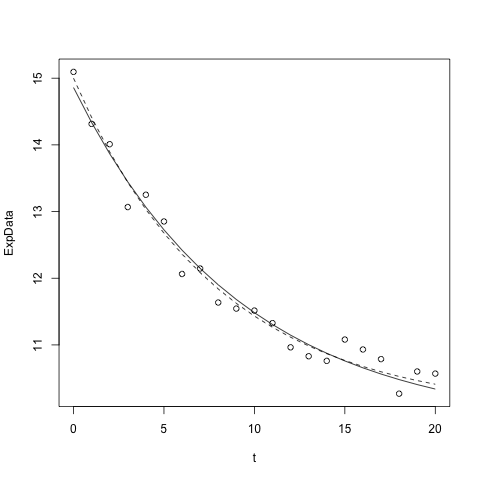
The R function lines works just like plot, but ADDS a line connecting points to the most recent plot. We can, for example, use our (previously defined above) function to add the theoretical ("noiseless") curve as a dashed line (see "line type" below):
lines(t,myExpDecay(t,5.0,8.0,10.0),lty="dashed")
Or we can ADD the best fit curve to the plot:
lines(t,myExpDecay(t, 4.63, 6.99, 10.34))
Note that you can similarly ADD data points to an existing plot
points(t, ExpDataMore, col="blue")
For advice on how to control axes, annotate plots, and more see our intermediate plotting in R, or for more, see this introduction and this reference.
There are many web sites that give you tips on advanced graphics options. You can plot two different sets of data using the same x-axis, but different y-axis scales.
Error Bars. We can ADD error bars to a plot using a more generic tool for drawing arrows.
arrows(x, y-sdev, x, y+sdev, length=0.05, angle=90, code=3)
Residuals. A plot of residuals (observed - best fit predicted, at each point) is valuable to look for systematic deviation. To plot residuals easily (in a new graph):
plot(t, residuals(model), main="Residuals", ylab="Residuals (predicted-experiment"))
When to use bar charts? As an aside, a word about two type of plots that might interest us: bar charts and x,y plots. Bar charts should only be used for data in which the x axis is "quantized" - categories, etc. x,y scatter plots should be used when the x-axis represents a continuous function. For example, you may have measured a time course at 1, 2, 3, 4, 5 ... min. Even though these are discrete values, the reaction continued (smoothly) between 1 and 2 min, etc. Bar charts are never appropriate for these data.
Output plots to PDF. To write a plot to a file, you need to 1) open an output "device," 2) execute the plot command(s), and 3) close the device - as in the example below, where we open the "pdf device" for output.
pdf("myPlot.pdf")
plot(t, ExpData)
dev.off()
In place of the single plot command, you can include a series of commands, line by line (for example, adding theoretical or best-fit curves, as above). Just be sure to end them with dev.off(), which writes the final result to the current working directory. Complete documentation for the PDF command can be found at RDocumentation.
[ Note that in RStudio, you can generate a plot, add to it, etc, and when you have it the way you want, you can then save it to PDF or Image (PNG) via Plots > Save as Image/PDF. Previous plots can be cycled through using the forward and backward arrow in the mini menu. ]
There are similar commands for writing to other formats: postscript("myPlot.ps"), svg("myPlot.svg"), png("myPlot.png"), and more. However, note that Powerpoint, Illustrator, and many other programs can insert PDF files, and this is strongly preferred over PNG, as
- the graphics will scale nicely
- the output will have no "jagged edges"
- you can edit the graph in Illustrator
If you must use a bitmapped image, PNG is much better suited to this type of graphics than is JPG.
If you want to edit your file in Illustrator (or Inkscape), some of the plotting point objects might look like letters instead of circles, squares, etc. To avoid this problem use:
pdf("myPlot.pdf", useDingbats=FALSE)
Quick navigation: Basics, Functions, Curve Fitting, Plotting, Importing Data, Files
Importing Data
To import data from a file, there are several options. We'll use the "data frame" formalism that includes multiple data vectors in one frame. Think of a single column in Excel as one such data vector, and an entire table as the data frame.
dataFrame <- read.csv("datafile.csv", header = FALSE)
The above command will take text data, such as that generated by an instrument or exported from Excel in CSV format (not native Excel), and read the data into a "data.frame" object (to read data directly from Excel files, see this tutorial). A more general command below uses sep= to specify that the data are "comma delimited":
dataFrame <- read.table("datafile.txt", sep=",", header = FALSE)
Columns in this table will have default headings V1, V2, etc. If the first line of your data file has heading information, then use
dataFrameH <- read.csv("datafileH.csv", header = TRUE)
Now the columns will adopt the names supplied in the first line. Simply type the name of the object (in this case, "dataFrameH", at the command line and you will get a print out of the data (be careful if your data set is large!). Example output (the first 5 lines) is
t decay x.square
1 0.0 1.000 0.0
2 0.5 0.779 0.3
3 1.0 0.607 1.0
4 1.5 0.472 2.3
5 2.0 0.368 4.0
The very first column (1, 2, 3, 4, 5) is not in the data; it's just row counters. The vector t is 0.0, 0.5, 1.0, ...; the vector decay is 1.000, 0.779, 0.607, ...
[ Note that in RStudio, you can import data via the menu File > Import Data Set ]
We can extract vectors by name, as in:
exptime <- dataFrameH$t
expdecay <- dataFrameH$decay
where $t and $decay specify those named vectors from our data.frame. The embedded vectors can also be used directly, as in
plot(dataFrameH$t, dataFrameH$decay)
A more object-oriented, and easier to read version of the same command is:
with(dataFrameH, plot(t, decay))
On a related note, should you want to write data to a CSV file, first it is easiest to put your data into a data.frame, using (include as many vectors as you like):
dfexport <- data.frame(t, ExpData)
To write that to a file:
write.csv(dfexport,"~/FileName.csv", row.names = FALSE)
Quick navigation: Basics, Functions, Curve Fitting, Plotting, Importing Data, Files
More on files, scripts, sessions
Saving and Reloading a Working Session. After importing data and setting some things up, might not want to have to re-do all of that. Therefore, you can save multiple "objects" (variables, functions, etc) generated during your session to a single file (specify as many as you like!), and then come back later and re-load those objects.
save(exptime, expdecay, dataFrameH, myExpDecay, file="myWork.rda")
You can then quit R, and come back, re-open R and use
load("myWork.rda")
and begin using exptime, expdecay, dataFrameH, myExpDecay, etc. Remember that in your second session, you need be in (see "setwd" above) your original working directory. To see a list of loaded objects, use the command ls()
[ Note that in RStudio, you can load and save sessions under the Session menu ]
Running scripts. Instead of typing, and re-typing commands, you can run a set of commands (a script) from a simple text file. Just place a series of commands in a file (saved as a text file, not a Word document, etc, and saved in your working directory). Use your favorite text editor - I recommend BBEdit (free version is fine) for Macs or Notepad for Windows. Then to run the entire script, simply enter the following in R:
source("scriptFile.txt")
In the same way that you can direct plotting output to a file, you can also direct screen (textual) output to a file. Simply precede those commands with:
sink("output.txt", append=FALSE, split=TRUE)
Now all output that would go to your screen will be directed to that file (text, not graphics). append=TRUE adds to the end of an existing file. split=TRUE sends output both to the file and to the screen. To stop future output from going to the file and return to the screen, use:
sink()
Quick navigation: Basics, Functions, Curve Fitting, Plotting, Importing Data, Files