R - Plotting Intermediate
This page assumes the basic introduction to plotting found in the introductory pages.
Intro plotting recap
Read this: the following assumes you are familiar with the basics of R. For a quick review, see this introduction to R. Other quick tidbits: the following creates a list of two numbers: c(1.0,3.5). See note below regarding "up arrow" uses.
Very quick review. Assuming you have equal lists of data in vectors x and y (defined t above), initiate a new graph using:
plot(x,y)
You can then ADD more lines or points using (as often as needed)
lines(x,y)
points(x,y)
Setting defaults up front
The examples in the next sections will assume that you set parameters during a plot, lines, or points call, but you can also set defaults with the command par before you issue a plots, lines, or points call. For example:
par(lwd=2, main="Plots in this set")
Customizing lines and symbols
These functions all take a wide range of modifiers in the call. We'll use "plot" as the example.
- Plot type: plot(x,y,type="l")
- type options are l (line), p (point), b (both) - and other fancy stuff
- Line Type: plot(x,y,lty="dashed")
- Line type options are: solid, dashed, dotted, dotdash, longdash, et al.
- Line width: plot(x,y,lwd=2)
- Numerical value, bigger is fatter (default=1)
- This also effects symbol thickness
- Color: plot(x,y,col="red")
- Color options are standard: red, blue, green, orange, magenta, olive, tan, purple, grey, black, white, ivory, and many more...
- Can also use numerical values
- Plot symbol (character): plot(x,y,pch=0)
- Open square (0), circle (1), diamond (5)
- Filled square (15), circle (16), diamond (18)
- See this list for more options. I have a mild bias against triangles and other symbols that are not uniformly symmetrical (harder for the reader to see where the symbol is centered), but use them when you exhaust the above (or use color!)
- Symbol size: plot(x,y,pch=0,cex=2)
- The size of plotted symbols. Default is 1. Fractional values OK.
Adding reference lines
In addition to plot, lines, and points, you can ADD straight reference (or other) lines to your plot using the command abline.
- Horizontal line: abline(h=3.14)
- Vertical line: abline(v=13)
- Arbitrary line: abline(a=53.1,b=2.2)
abline takes the following arguments, in addition to the arguments described above for plot, lines, and points (lty, col, lwd, etc)
- a: intercept
- b: slope
- h: y-value for a horizontal line
- v: x-value for a vertical line
The following parameters can be added to the initial plot call
Labels
- Plot title: plot(x,y,main="The big picture plot title")
- Plot subtitle: plot(x,y,sub="the sub-title")
- x-axis label: plot(x,y,xlab="Ligand concentration (µM)")
- y-axis label: plot(x,y,ylab="Fluorescence (arbitrary units)")
You can specify font sizes and colors for any of these (though this is reportedly somewhat dependent on your OS), following these examples:
- Font size: plot(x,y,cex=1.5)
- Increases font size to 150% throughout
- To change only certain regions:
- Plot title: plot(x,y,main="The big picture plot title")
- Plot subtitle: plot(x,y,sub="the sub-title")
- x-axis label: plot(x,y,xlab="Ligand concentration (µM)")
- y-axis label: plot(x,y,ylab="Fluorescence (arbitrary units)")
- cex.lab - axis labels, cex.axis - axis tick mark annotations,
- Font color: as above, e.g. plot(x,y,col.lab="blue")
- Font style: as above, e.g. plot(x,y,font.main="bold")
- 1: plain text; 2: bold; 3: italic; 4:bold italic
- Font family: as above, e.g. plot(x,y,family.axis="sans")
- Options include: mono, sans, serif, et al.
For publications, it's always best to import your final figure into Illustrator. There you can very easily add and edit text on your graph (never edit the data!).
To add a legend to your plot, with the bottom left at x=0, y=1.2 (plot units):
- legend(0, 1.2, c("Lbl1", "Lbl2", "Lbl3"), lty = c("solid","dashed","dotted"), col = c("red", "blue", "green")
Axis limits
To override having R pick your limits for you, you can include the following:
- x-axis limits: plot(x,y,xlim=c(-0.5,2.5))
- y-axis limits: plot(x,y,ylim=c(10.0,50.0))
- log scale: plot(x,y,log="x")
- options include x, y, xy (or yx) to specify which axes are log scale
For still more control over axes, see this introduction and this reference.
There are many web sites that give you tips on advanced graphics options. You can plot two different sets of data using the same x-axis, but different y-axis scales.
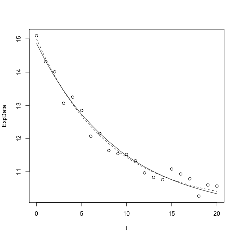
Tips for use with fitting data to models
If you have just fit a model to data with nls, as in the example below
model1 <- nls(fluorI ~ eDecay(t,myA,myT), data=ExpData, start=list(myA=10,myT=5))
and have previously plotted the data as points, you can plot the best fit curve using
lines(ExpData$t,predict(model1)
However, unless you have many, tightly spaced data points, the curve may not be as smooth as you'd like and you may want to plot the curve outside of the data range a bit (the above plots only at the t values that were fit).
To have more control over the presentation of your best fit curve, define a new x-axis range using either of the following
tt <- seq(0, 10, by = 0.5)
tt <- seq(0,10, length=21)
and then call the original function with the best fit parameters
lines(tt,eDecay(tt, 3.1, 5.22))
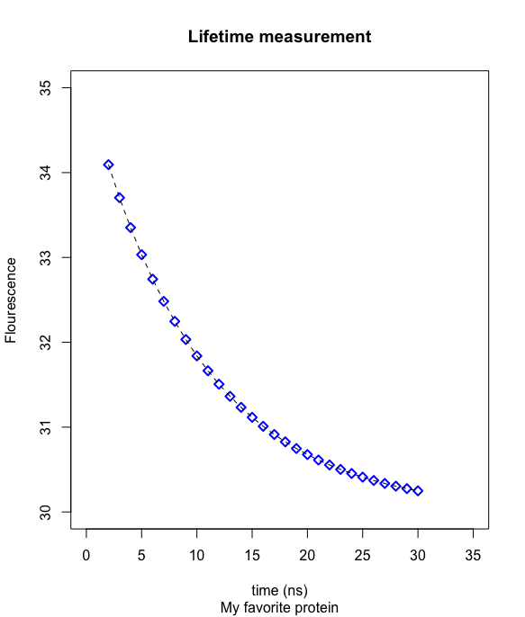
Setting default plotting values
The par command lets you specify many of the above things up front, to apply, by default, to subsequent plot, lines, and points calls.
Example
- plot(x,y,type="p",pch=5,col="blue",lwd=2,main="Lifetime measurement",sub="My favorite protein",ylab="Flourescence",xlab="time (ns)",xlim=c(0,35),ylim=c(30,36))
- lines(x,y,type="l",lty="dashed",col="black")
Important: you will almost certainly experience typos that corrupt your initial command and you'll get an error message from R. You might have to just change one thing, but you don't want to re-type the command. Here, the "up arrow" key on your keyboard is essential. All of your prior commands are stored, and you can retrieve any simply by hitting the "upper arrow" key as many times as you need (and if you over-shoot, use the down arrow command). You can then edit the old command and then press "return" to execute the revised command.