R - fitting data to a mathematical model
Nonlinear Least Square Curve Fitting
-- this page assumes familiarity with a basic intro to R --
The R function nls (nonlinear least squares) optimizes parameters of a user function to fit that function to experimental data (see detailed documentation here). The following illustrates its use (and see this nice overview).
Read in experimental data. To illustrate the approach, we'll start with some experimental data - download the data here if you want to play along. As described in a basic intro to R we can load that data into an R data frame using:
ExpData <- read.csv("ExpDataRTutorial.csv", header = TRUE)
We will use two columns (vectors) from that data: t (time in ns) and fluorI (fluorescence intensity). To examine the data, use the plot command described in a basic intro to R.
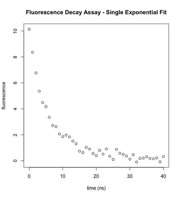
plot(ExpData$t,ExpData$fluorI,xlab="time (ns)", ylab="fluorescence",main="Fluorescence Decay Assay - Single Exponential Fit")
Note that we can extract data "vectors" out of the ExpData frame using their column headings: t and flourI.
Inspect the data. Visual inspection of the data confirms an apparent exponential decay. Moreover, we can estimate a few things that will be useful at the next step. The starting intensity looks like it's around 10-11 fluorescence units. It's half-maximal value is at about 5 nsec, very approximately. But we want much more than that.
Define a function to fit data to. We know that the data are from a fluorescence lifetime measurement and so we expect the data to follow an exponential decay: \(F=Ae^{-t/\tau }\). Thus we will want to define a corresponding R function
eDecay <- function(t, ampl, tau) (ampl*exp(-t/tau))
This function defines an exponential decay with starting amplitude "ampl" and following a decay lifetime of "tau"
nls - a nonlinear least squares fitting function in R. The basic nonlinear least squares fitting function in R takes the form
nls( ExpData ~ TheoryFunction, data=DataFrame, parameter initial guesses)
In this case, ExpData ~ TheoryFunction instructs the algorithm to compare experimental data to theoretical data (while varying the parameters that define the theoretical function. Dataframe is the table we read in that contains the data. Finally, we need to tell the algorithm a reasonable list of starting guesses for the parameters (with a good data and function match, the guesses shouldn't have to be very good).
The goal of nonlinear least squares fitting algorithms is to find function parameters that minimize the residual sum of squares (more on residuals, below), in other words the agreement between theory and experiment.
$$\begin{aligned}RSS=\sum \left( obs-pred\right)^2 \end{aligned}$$
Specifying a fit. The actual one-line code to carry out the fit of the data in myExpData to the function myExpDecay is the following. Note that we must supply starting guesses. From our visual inspection above, we'll use ampl=10 and tau=5.
nls(fluorI ~ eDecay(t,myA,myT), data=ExpData, start=list(myA=10,myT=5))
Remember that dat and t are data vectors in ExpData. This says that the function eDecay intends to predict dat (our y-value) based on t (our x-value) and the parameters myA and myT.
Nonlinear regression model
model: fluorI ~ eDecay(t, myA, myT)
data: ExpData
myA myT
9.524 6.270
residual sum-of-squares: 4.35
Number of iterations to convergence: 7
Achieved convergence tolerance: 5.514e-06
The above will print some basic results, but let's modify the command slightly to store the fit results in an R object named model1 (a number of R functions know how to access those results and we will use some below. Some of the functions that let you look inside the result include summary, confint, predict, residuals, anova, coef, deviance, df.residual, fitted,formula, logLik, predict, print, profile, vcov and weights.
model1 <- nls(fluorI ~ eDecay(t,myA,myT), data=ExpData, start=list(myA=10,myT=5))
After this call, the variable model1 is now loaded with the results of the fit. To display a summary of the fit, use (in a script, you might have to call: print(summary(model1)):
summary(model1)
The output should look like (bold formatting added for emphasis):
Formula: fluorI ~ eDecay(t, myA, myT)
Parameters:
Estimate Std. Error t value Pr(>|t|)
myA 9.5239 0.2294 41.52 <2e-16 ***
myT 6.2702 0.2308 27.16 <2e-16 ***
---
Signif. codes: 0 ‘***’ 0.001 ‘**’ 0.01 ‘*’ 0.05 ‘.’ 0.1 ‘ ’ 1
Residual standard error: 0.334 on 39 degrees of freedom
Number of iterations to convergence: 7
Achieved convergence tolerance: 5.514e-06
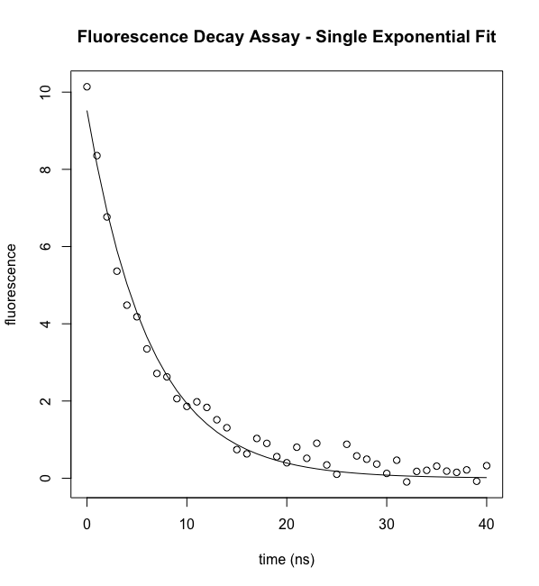
The best fit parameter estimations are Ampl = 9.52 ± 0.23 and tau = 6.27 ± 0.23 ns (remember that this parameter has units of time that match those of the experimental time). Uncertainties listed are the standard error of each parameter (more on that below).
Note that we could generate the "best fit" y-values by substituting the best fit parameters in our function:
fitY <- eDecay(ExpData$t, 9.52, 6.27)
or equivalently, we can use a built in function that uses the information stored in model1.
fitY <- predict(model1)
To plot the experimental data, then the best fit curve:
plot(ExpData$t,ExpData$fluorI,xlab="time (ns)", ylab="fluorescence",main="Fluorescence Decay Assay - Single Exponential Fit")

lines(t,predict(model))
The function predict() is convenient for plotting the best fit curve. However, it only includes as many points as there are data points and so for fits with relatively few data points, the best fit "curve" will not be smooth. Note that you can access the best fit parameters using the following:
cc <- coef(model)
Afit <- cc["myA"]
Tfit <- cc["myT"]
You could then plot your theoretical curve as follows:
tfine <- 0.1*c(0:400)
lines(tfine,eDecay(tfine,Afit,Tfit)
The first line defines a more closely spaced set of time points (0 to 40 nsec, in 0.1 ns intervals). The second then draws lines between the predicted fluorescence for each of these points, using the best fit parameters.
One might look at the fit and decide that we are done. In results not shown, we repeated the measurement 3 more times and obtained data and best fit results that are very similar to those reports above. So we have reproducibility. Do we have rigor? No.
In any fit, one should always analyze fit residuals.
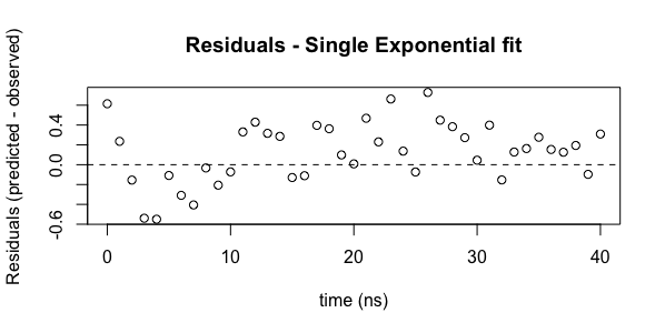
Assessment of fit quality - residuals. At any given point the residual is defined as (best fit predicted - observed). For a perfect fit, these would be zero, but we never have a perfect fit. As noted above, what we really want to assure is that the distribution of residuals is random. Plotting the residuals is a good way of carrying out this analysis and R makes this easy through a built in function to return these values. To plot residuals vs the independent variable (t, here):
plot(ExpData$t, residuals(model1), main="Residuals - Single Exponential fit", xlab="time (ns)", ylab="Residuals (predicted - observed)")

abline(h=c(0.0), lty=2)
In this case, the second command draws a horizontal line at 0.0, which is useful for examine the distribution around zero.
Looking at the residuals plot, we can see that the residuals are not randomly distributed. From 2-10 ns, all values are less than zero. Beyond 10 ns, almost all values are above zero. There is a systematic deviation in the residuals. Remember that the best fit parameters and the error analysis assume a normal distribution of the residuals.
What might be happening here? We know that fluorescent molecules can have more than one excited state and therefore more than one relaxation time. Looking at the fluorescence plot, we can see an initial drop that is a bit faster than the curve predicts and the long time point data don't reach zero as quickly as the equation predicts. We hypothesize that there might be two decays happening. So let's generate an equation for a biexponential decay.
$$\begin{aligned}F=A\left( \left( 1-f\right) _{et}^{-t/\tau _{1}} + f_{e}^{-t/\tau _{2}}\right) \end{aligned}$$
eDecay2 <- function(t, ampl, f1, tau1, tau2) (ampl*((f1*exp(-t/tau1))+((1-f1)*exp(-t/tau2))))
We can then re-fit the data using the above
model2 <- nls(fluorI ~ eDecay2(t,myA,myf,myTau1,myTau2), data=ExpData, start=list(myA=10, myf=0.5, myTau1=2.5, myTau2=10))
Evaluating the results, we get
summary(model2)
Formula: fluorI ~ eDecay2(t, myA, myf, myTau1, myTau2)
Parameters:
Estimate Std. Error t value Pr(>|t|)
myA 10.1816 0.1912 53.241 < 2e-16 ***
myf 0.6374 0.1074 5.933 7.75e-07 ***
myTau1 3.4062 0.5409 6.297 2.49e-07 ***
myTau2 11.8507 2.0367 5.818 1.11e-06 ***
---
Signif. codes: 0 ‘***’ 0.001 ‘**’ 0.01 ‘*’ 0.05 ‘.’ 0.1 ‘ ’ 1
Residual standard error: 0.2157 on 37 degrees of freedom
Number of iterations to convergence: 5
Achieved convergence tolerance: 9.086e-06
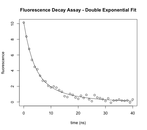
As above, we can plot the data vs the best fit.
plot(ExpData$t,ExpData$fluorI,xlab="time (ns)", ylab="fluorescence",main="Fluorescence Decay Assay - Double Exponential Fit")
lines(ExpData$t,predict(model2))
And similarly, we can generate the residuals plot
plot(ExpData$t, residuals(model2), main="Residuals - Double Exponential fit", xlab="time (ns)", ylab="Residuals (predicted - observed)")
abline(h=c(0.0), lty=2)
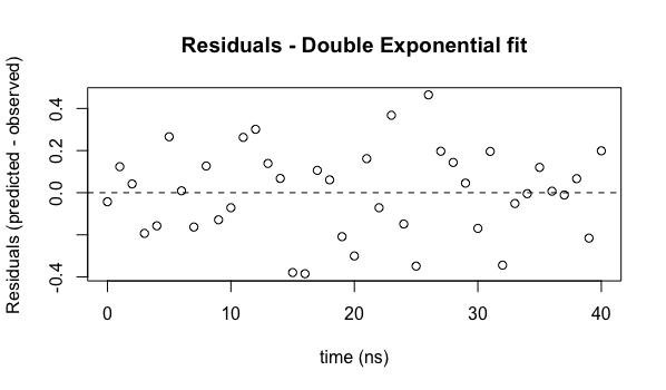
We now see that the residuals do not appear to have any systematic behavior - they are distributed reasonably uniformly (and their magnitudes are smaller, indicating a better fit of the model to the data).
You should always generate and analyze a residuals plot (publishing it alongside your best fit will convince people that you know what you are doing!).
Standard errors of the fit parameters. Now that we are reasonably convinced that we are using the correct model, we can proceed to analyze the parameters and their uncertainties. From the summary(model2) results, we have found
- myA = 10.18 ± 0.19 (Amplitude)
- myf = 0.64 ± 0.11 (fraction contribution from tau1)
- myTau1 = 3.41 ± 0.54 (Tau1 - decay lifetime)
- myTau2 = 11.8 ± 2.0 (Tau2 - decay lifetime)
The "plus/minus" uncertainties reported by R are the "standard error" around each best fit parameter. The estimate, assuming a number of things, is that we can be 95% confidence that the actual parameter lies within two standard errors of the fitted parameter (actually, standard error reports the expected precision of the determination). Thus the actual amplitude at time zero has a 95% chance of lying in the range 9.8...10.6.
Confidence intervals. In some cases this is OK, but for fits to nonlinear equations, such as this, there is no reason for the uncertainties to be symmetrically distributed around the best fit value. So instead, we can ask R to report confidence intervals of the fit parameters, using the following:
confint(model2, level=0.95)
2.5% 97.5%
myA 9.7955298 10.5787091
myf 0.4122709 0.8441233
myTau1 2.2799537 4.5463496
myTau2 8.8830769 20.0278058
So for the uncertainty in the amplitude, this agrees with the simpler analysis. For all fit parameters, the 95% confidence intervals are compared (in parentheses) with what one can calculate from ± 2 x Std Err.
| myTau2 ± 2(Std Err) | 95% Conf Intrvl | |
| myA | 9.8 ... 10.6 | 9.8 ... 10.6 |
| myf | 0.41 ... 0.84 | 0.42 ... 0.86 |
| myTau1 | 2.3 ... 4.5 | 2.3 ... 4.5 |
| myTau2 | 8.9 ... 20.0 | 7.8 ... 15.8 |
Note that the spread of uncertainty that we get using ± 2 x standard error (which corresponds approximately to a 95% confidence interval) is close, but not identical to the confidence interval. Also note that for myTau2, the confidence interval around the estimated parameter is not fully symmetrical, as we guessed that it might not be.
The following pair of commands generates a series of plots, one for each fit parameter, showing the parameter confidence intervals as a function of the level of confidence.
pf=profile(model2)
plot(pf, conf = c( 99, 95, 90, 80, 50)/100,  absVal = TRUE, ylab = NULL, lty = 2)
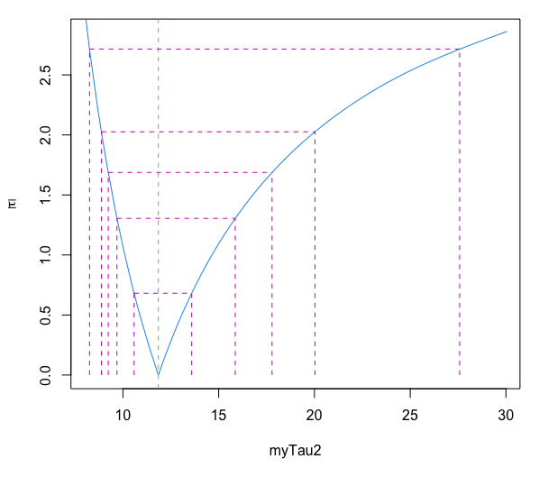
This clearly illustrates the asymmetry in the uncertainty range around the best fit value of 11.8 ns.
Note that with only 50% confidence, you can say that the actual value of tau2 is in the range 10.5...13.6 (the innermost range). But to be 99% confidence that the actual value of tau2 is in a specified range, you to have to expand the confidence interval to 8.3...27 (the outermost range).
When you report uncertainties in manuscripts and dissertations, you should always be very explicit about what you are reporting. 95% confidence intervals are ideal.
Note also that this plot shows that our uncertainty in tau2 is not symmetric, as the simple ± representation incorrectly suggests.
Interdependence of parameters. In estimating the fit to a function, analysis of more things hidden in the results can tell us about interdependence of parameters in the fit - in other words, changing one parameter may lead to a more poor fit, but changing a different parameter can bring the quality of the fit back. The following R command yields the variance - covariance matrix:
vcov(model)
myA myf myTau1 myTau2
myA 0.036570721 -0.004941673 -0.04908717 -0.09500579
myf -0.004941673 0.011544136 0.05370280 0.21196610
myTau1 -0.049087171 0.053702797 0.29258897 0.94422084
myTau2 -0.095005790 0.211966099 0.94422084 4.14823095
The diagonal entries are the variance of each parameter (self-covariance). The value of -0.09500579 is the covariance between parameters myA and myTau2. While all of these terms have statistical meaning, their more easily interpreted counterparts are correlation coefficients - normalized versions of covariance.
Correlation coefficients are a normalized approach to looking at how parameters impact each other. In R, one can retrieve correlation coefficients using:
summary(model,correlation=TRUE)
Correlation of Parameter Estimates:
myA myf myTau1
myf -0.24
myTau1 -0.47 0.92
myTau2 -0.24 0.97 0.86
This is just one corner of the more complete correlation matrix. Noting the symmetry, you can manually regenerate the more complete matrix by hand.
Correlation of Parameter Estimates:
myA myf myTau1 myTau2
myA 1.00 -0.24 -0.47 -0.24
myf -0.24 1.00 0.92 0.97
myTau1 -0.47 0.92 1.00 0.86
myTau2 -0.24 0.97 0.86 1.00
The values of a correlation coefficient range from -1 to +1, where 0 indicates no correlation between two parameters. The above correlation matrix says that myA correlates fully with myA (of course), but correlates inversely with the other parameters, some more than others. It raises warning flags about correlation/covariance between the parameters myf and both myTau1 and myTau2, and raises some concern regarding correlation of myTau1 and myTau2. These relationships may indicate a problem with the model (though often the model itself imparts inter-dependence of variables).
What about the p-value? Note that for the above parameters, R reports out Pr(>|t|), the p-value, for each parameter. This is not particularly useful in the current example. The p-value is the probability of obtaining the observed test results under the assumption that the null hypothesis is correct. A small p-value indicates that it is unlikely we will observe a relationship between the measured observation (fluorescence signal here) and each parameter due to random chance. It does not tell us that this model is correct or that there is not a better model. In this regard, the p-value is often misused.
What about the t-value? The t-value is a measure of how many standard deviations our coefficient estimate is from 0. It is related to the p-value and is similarly not particularly useful in this case, for the same reasons.
Comparing models. Assume that I have fit the same data with two different mathematical models and loaded the nls results in model1 and model2, respectively. How do I assess which is better?
anova(model1,model2)
Analysis of Variance Table
Model 1: fluorI ~ eDecay(t, myA, myT)
Model 2: fluorI ~ eDecay2(t, myA, myf, myTau1, myTau2)
Res.Df Res.Sum Sq Df Sum Sq F value Pr(>F)
1 39 4.3503
2 37 1.7210 2 2.6294 28.265 3.541e-08 ***
---
Signif. codes: 0 ‘***’ 0.001 ‘**’ 0.01 ‘*’ 0.05 ‘.’ 0.1 ‘ ’ 1
In the case of this Anova test, the p-value is useful. The small P-value (3e-8) tells us that the models are (statistically) significantly different (the biexponential decay model with the smaller residual sum of squares is statistically better than the single exponential).
What is the biggest mistake people make in interpreting fits? The error analysis, specifically the standard error for each parameter, assumes that the underlying data follow the model perfectly and that the "noise" in the data are distributed according to the "normal" function. Nature is rarely as "perfect" as we like, and even if it is, we often are not. Errors might arise from pipetting errors and we may have a tendency, for example, to under-pipette more than over-pipette - a systematic error. In preparing the experiment, we may have determined the protein concentration, for example and then used that throughout. If that concentration is off, then our best fit parameters will be incorrect (or at least, more uncertain). The data may be following our model mostly, but with a minor contribution from a process we are not aware of (our protein is sticking to surfaces or aggregating over time, for example). Thus a parameter that reports out as 11.8 ± 2.0 (or 11.8 with a confidence interval of 8.9...20) may be still less certain than we think. We may repeat the experiment and get 10.7 ± 1.8 and congratulate ourselves on the accuracy of our assay. If there is a systematic error, both numbers may be different from the real value, in the same way. We have achieved precision (reproducibility), but not accuracy.
Always do a "gut" test: do I really believe that the parameter is as certain as the program reports?
Whenever possible, seek a second opinion. Is there a way to get one or more of these parameters from a completely different measurement (not subject to the same types of "noise" as my current assay). Or at least do a test that will come out measurably different if your conclusions are not correct.
What about the other summary stuff? For more, this web page focused on fitting a linear model, gives a nice explanation of each part of the output (though some parts are specific to the linear fitting).
I'm getting a "singularity" error. It is up to you to see that your equation doesn't include redundancies or ambiguities, for the data you are fitting. For example, consider the equation for a biexponential that we used above
$$\begin{aligned}F=A\left( \left( 1-f\right) _{et}^{-t/\tau _{1}} + f_{e}^{-t/\tau _{2}}\right) \end{aligned}$$
with fit parameters A, f, tau1, and tau2. If your data are biexponential, this equation should fit well. However, if your data represent a single exponential, such that tau1=tau2. In this case, ANY value of f will yield the same value of F. The algorithm will not be able to fit the function at all and will report an error (usually referencing a "singularity"). More broadly, trying to fit an equation with insufficient data can lead to similar errors. This is true in any program trying to do nonlinear regression, not just nls in R.
Advanced topics
Plotting pairwise confidence intervals. We saw above that there are interdependencies between parameters in a complex function. The correlation matrix told us about this. To see more clearly how one parameter depends on another we can add an external "package" to R, using the install command, and then activate a function in that package using the library command. (you should only have to install once; you may need to call library in each new R session).
install.packages("ellipse")
library("ellipse")
In RStudio, you can also add packages by clicking on the "Packages" tab (generally in the same box as "Plots"). Then click on the "Install" button. Using the standard (CRAN) repository, ask to install the "ellipse" package. In the User Library listing that follows, check the box next to "ellipse" (confusingly, ellipse is a function within the ellipse package).
Next, for an nls fit model2, to plot the interdependency between any two parameters at the 95% confidence interval, use:
plot(ellipse(model2,level=c(0.95),which=c('myTau1','myTau2')), type = 'l')
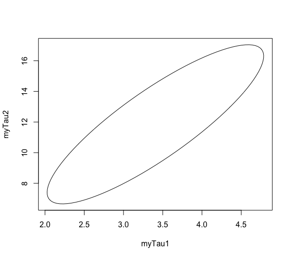
This plot shows that any combination of tau1 and tau2 that lies within the ellipse falls within the 95% confidence interval for this fit. We are 95% confident (and assuming all of our other assumptions) that any of those values could reflect the true behavior of the system. It illustrates that the two parameters are interdependent.
It is not uncommon to add other confidence levels by graphing lines in the same plot
lines(ellipse(model2,level=c(0.90),which=c('tau1','tau2')), type = 'l')
To generate your own simulated experimental data. Start by generating the x-axis (independent variable) part of the data, in this case time:
t <- 0:20
This creates a vector [0, 1, 2, ..., 20]. We'll now use our myExpDecay function to generate some simulated experimental data, complete with normally distributed noise.
ExpData <- myExpDecay(t,5.0,8.0,10.0) + rnorm(21,mean=0,sd=0.2)
The first half of the above takes the 21 length time vector and generates a 21 length vector with signal that decays according to the specified parameters. The second half generates a 21 length vector with normally distributed random noise. The two vectors are added together to generate data with random noise.
Simulating Chemical Kinetics
With the speed of modern computers and simple software packages in R (and other environments) it is now possible to easily simulate any complex chemical or enzymological reaction. And of course, if we can simulate the process, we can fit data. The process for doing this is called numerical integration. Consider the process A -> B, as in fluorescence decay.
$$\begin{aligned}A\xrightarrow{k}B\end{aligned}$$
We know from introductory chemistry classes that we can write the rate of decrease in concentration of A as
$$\begin{aligned}\dfrac{-d\left[A\right] }{dt} = k\left[A\right]\end{aligned}$$
We know from introductory calculus classes that we can rearrange the above to
$$\begin{aligned}-d\left[A\right] = k\left[A\right]dt\end{aligned}$$
$$\begin{aligned}\int_{0}^{t}d\left[A\right]\,dt = -k \int_{0}^{t}\left[A\right]dt\end{aligned}$$
and that we can solve that integral explicitly to yield
$$\begin{aligned}A_{t}=A_{0}e^{-kt }\end{aligned}$$
Note that we can also integrate a function by determine the area under the curve, a small step at a time. Mathematically, this looks like
$$\begin{aligned}\left[A\right]_{t_{i}}=\int_{0}^{t_{i}}d\left[A\right]\,dt = \left[A\right]_{t_{0}} + \sum_{t=0}^{t=t_{i}}-k\left[A\right]_{t}\Delta t\end{aligned}$$
In the above, at any given point in time, $-k\left[A\right]_{t}$ is the rate of change of A and $-k\left[A\right]_{t}\Delta t$ is the amount A changes over time $\Delta t$. This approach can be used for equations that cannot be simply solved analytically as above. This approach can also be used for systems of coupled differential equations.
Consider the slightly more complex reaction
$$\begin{aligned}A\xrightarrow{k_{a}}B\xrightarrow{k_{b}}C\end{aligned}$$
We can write the rate expressions as:
$$\begin{aligned}\left[A\right]_{t_{i}}= \left[A\right]_{t_{0}} + \sum_{t=0}^{t=t_{i}}-k_{a}\left[A\right]_{t}\Delta t\end{aligned}$$
$$\begin{aligned}\left[B\right]_{t_{i}}= \left[B\right]_{t_{0}} + \sum_{t=0}^{t=t_{i}}\left\{k_{a}\left[A\right]_{t} - k_{b}\left[B\right]_{t}\right\}\Delta t\end{aligned}$$
$$\begin{aligned}\left[C\right]_{t_{i}}= \left[C\right]_{t_{0}} + \sum_{t=0}^{t=t_{i}}k_{b}\left[B\right]_{t}\Delta t\end{aligned}$$
Download this script for a template for simulating kinetics of complex reactions. But first, you'll need to install a package for ordinary differential equations:
install.packages("deSolve")
library(deSolve)
library(ode)
mglksjfdglk